# Implementation of Maximum Weighted Matching
## Introduction
This document describes the implementation of an algorithm that computes a maximum weight matching
in a general graph in time _O(n3)_, where _n_ is the number of vertices in the graph.
In graph theory, a _matching_ is a subset of edges such that none of them share a common vertex.
A _maximum cardinality matching_ is a matching that contains the largest possible number of edges
(or equivalently, the largest possible number of vertices).
For a graph that has weights attached to its edges, a _maximum weight matching_
is a matching that achieves the largest possible sum of weights of matched edges.
An algorithm for maximum weight matching can obviously also be used to calculate a maximum
cardinality matching by simply assigning weight 1 to all edges.
Certain computer science problems can be understood as _restrictions_ of maximum weighted matching
in general graphs.
Examples are: maximum matching in bipartite graphs, maximum cardinality matching in general graphs,
and maximum weighted matching in general graphs with edge weights limited to integers
in a certain range.
Clearly, an algorithm for maximum weighted matching in general graphs also solves
all of these restricted problems.
However, some of the restricted problems can be solved with algorithms that are simpler and/or
faster than the known algorithms for the general problem.
The rest of this document does not consider restricted problems.
My focus is purely on maximum weighted matching in general graphs.
In this document, _n_ refers to the number of vertices and _m_ refers to the number of edges in the graph.
## A timeline of matching algorithms
In 1963, Jack Edmonds published the first polynomial-time algorithm for maximum matching in
general graphs [[1]](#edmonds1965a) [[2]](#edmonds1965b) .
Efficient algorithms for bipartite graphs were already known at the time, but generalizations
to non-bipartite graphs would tend to require an exponential number of steps.
Edmonds solved this by explicitly detecting _blossoms_ (odd-length alternating cycles) and
adding special treatment for them.
He also introduced a linear programming technique to handle weighted matching.
The resulting maximum weighted matching algorithm runs in time _O(n4)_.
In 1973, Harold N. Gabow published a maximum weighted matching algorithm that runs in
time _O(n3)_ [[3]](#gabow1974) .
It is based on the ideas of Edmonds, but uses different data structures to reduce the amount
of work.
In 1983, Galil, Micali and Gabow published a maximum weighted matching algorithm that runs in
time _O(n\*m\*log(n))_ [[4]](#galil_micali_gabow1986) .
It is an implementation of Edmonds' blossom algorithm that uses advanced data structures
to speed up critical parts of the algorithm.
This algorithm is asymptotically faster than _O(n3)_ for sparse graphs,
but slower for highly dense graphs.
In 1983, Zvi Galil published an overview of algorithms for 4 variants of the matching problem
[[5]](#galil1986) :
maximum-cardinality resp. maximum-weight matching in bipartite resp. general graphs.
I like this paper a lot.
It explains the algorithms from first principles and can be understood without prior knowledge
of the literature.
The paper describes a maximum weighted matching algorithm that is similar to Edmonds'
blossom algorithm, but carefully implemented to run in time _O(n3)_.
It then sketches how advanced data structures can be added to arrive at the Galil-Micali-Gabow
algorithm that runs in time _O(n\*m\*log(n))_.
In 1990, Gabow published a maximum weighted matching algorithm that runs in time
_O(n\*m + n2\*log(n))_ [[6]](#gabow1990) .
It uses several advanced data structures, including Fibonacci heaps.
Unfortunately I don't understand this algorithm at all.
## Choosing an algorithm
I selected the _O(n3)_ variant of Edmonds' blossom algorithm as described by
Galil [[5]](#galil1986) .
This algorithm is usually credited to Gabow [[3]](#gabow1974), but I find the description
in [[5]](#galil1986) easier to understand.
This is generally a fine algorithm.
One of its strengths is that it is relatively easy to understand, especially compared
to the more recent algorithms.
Its run time is asymptotically optimal for complete graphs (graphs that have an edge
between every pair of vertices).
On the other hand, the algorithm is suboptimal for sparse graphs.
It is possible to construct highly sparse graphs, having _m = O(n)_,
that cause this algorithm to perform _Θ(n3)_ steps.
In such cases the Galil-Micali-Gabow algorithm would be significantly faster.
Then again, there is a question of how important the worst case is for practical applications.
I suspect that the simple algorithm typically needs only about _O(n\*m)_ steps when running
on random sparse graphs with random weights, i.e. much faster than its worst case bound.
After trading off these properties, I decided that I prefer an algorithm that is understandable
and has decent performance, over an algorithm that is faster in specific cases but also
significantly more complicated.
## Description of the algorithm
My implementation closely follows the description by Zvi Galil in [[5]](#galil1986) .
I recommend to read that paper before diving into my description below.
The paper explains the algorithm in depth and shows how it relates to matching
in bipartite graphs and non-weighted graphs.
There are subtle aspects to the algorithm that are tricky to implement correctly but are
mentioned only briefly in the paper.
In this section, I describe the algorithm from my own perspective:
a programmer struggling to implement the algorithm correctly.
My goal is only to describe the algorithm, not to prove its correctness.
### Basic concepts
An edge-weighted, undirected graph _G_ consists of a set _V_ of _n_ vertices and a set _E_
of _m_ edges.
Vertices are represented by non-negative integers from _0_ to _n-1_: _V = { 0, 1, ..., n-1 }_
Edges are represented by tuples: _E = { (x, y, w), ... }_
where the edge _(x, y, w)_ is incident on vertices _x_ and _y_ and has weight _w_.
The order of vertices is irrelevant, i.e. _(x, y, w)_ and _(y, x, w)_ represent the same edge.
Edge weights may be integers or floating point numbers.
There can be at most one edge between any pair of vertices.
A vertex can not have an edge to itself.
A matching is a subset of edges without any pair of edges sharing a common vertex.
An edge is matched if it is part of the matching, otherwise it is unmatched.
A vertex is matched if it is incident to an edge in the matching, otherwise it is unmatched.
An alternating path is a simple path that alternates between matched and unmatched edges.
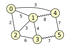
*Figure 1*
Figure 1 depicts a graph with 6 vertices and 9 edges.
Wavy lines represent matched edges; straight lines represent edges that are currently unmatched.
The matching has weight 8 + 7 = 15.
An example of an alternating path would be 0 - 1 - 4 - 5 - 3 (but there are many others).
### Augmenting paths
An augmenting path is an alternating path that begins and ends in two unmatched vertices.
An augmenting path can be used to extend the matching as follows:
remove all matched edges on the augmenting path from the matching,
and add all previously unmatched edges on the augmenting path to the matching.
The result is again a valid matching, and the number of matched edges has increased by one.
The matching in figure 1 above has several augmenting paths.
For example, the edge from vertex 0 to vertex 2 is by itself an augmenting path.
Augmenting along this path would increase the weight of the matching by 2.
Another augmenting path is 0 - 1 - 4 - 5 - 3 - 2, which would increase the weight of
the matching by 3.
Finally, 0 - 4 - 1 - 2 is also an augmenting path, but it would decrease the weight
of the matching by 2.
### Main algorithm
Our algorithm to compute a maximum weighted matching is as follows:
- Start with an empty matching (all edges unmatched).
- Repeat the following steps:
- Find an augmenting path that provides the largest possible increase of the weight of
the matching.
- If there is no augmenting path that increases the weight of the matching,
end the algorithm.
The current matching is a maximum-weight matching.
- Otherwise, use the augmenting path to update the matching.
- Continue by searching for another augmenting path, etc.
This algorithm ends when there are no more augmenting paths that increase the weight
of the matching.
In some cases, there may still be augmenting paths which do not increase the weight of the matching,
implying that the maximum-weight matching has fewer edges than the maximum cardinality matching.
Every iteration of the main loop is called a _stage_.
Note that the final matching contains at most _n/2_ edges, therefore the algorithm
performs at most _n/2_ stages.
The only remaining challenge is finding an augmenting path.
Specifically, finding an augmenting path that increases the weight of the matching
as much as possible.
### Blossoms
A blossom is an odd-length cycle that alternates between matched and unmatched edges.
Such cycles complicate the search for augmenting paths.
To overcome these problems, blossoms must be treated specially.
The trick is to temporarily replace the vertices and edges that are part of the blossom
by a single super-vertex.
This is called _shrinking_ the blossom.
The search for an augmenting path then continues in the modified graph in which
the odd-length cycle no longer exists.
It may later become necessary to _expand_ the blossom (undo the shrinking step).
For example, the cycle 0 - 1 - 4 - 0 in figure 1 above is an odd-length alternating cycle,
and therefore a candidate to become a blossom.
In practice, we do not remove vertices or edges from the graph while shrinking a blossom.
Instead the graph is left unchanged, but a separate data structure keeps track of blossoms
and which vertices are contained in which blossoms.
A graph can contain many blossoms.
Furthermore, after shrinking a blossom, that blossom can become a sub-blossom
in a bigger blossom.
Figure 2 depicts a graph with several nested blossoms.

*Figure 2: Nested blossoms*
To describe the algorithm unambiguously, we need precise definitions:
* A _blossom_ is either a single vertex, or an odd-length alternating cycle of _sub-blossoms_.
* A _non-trivial blossom_ is a blossom that is not a single vertex.
* A _top-level blossom_ is a blossom that is not contained inside another blossom.
It can also be a single vertex which is not part of any blossom.
* The _base vertex_ of a blossom is the only vertex in the blossom that is not matched
to another vertex in the same blossom.
The base vertex is either unmatched, or matched to a vertex outside the blossom.
In a single-vertex blossom, its only vertex is the base vertex.
In a non-trivial blossom, the base vertex is equal to the base vertex of the unique sub-blossom
that begins and ends the alternating cycle.
* The _parent_ of a non-top-level blossom is the directly enclosing blossom in which
it occurs as a sub-blossom.
Top-level blossoms do not have parents.
Non-trivial blossoms are created by shrinking and destroyed by expanding.
These are explicit steps of the algorithm.
This implies that _not_ every odd-length alternating cycle is a blossom.
The algorithm decides which cycles are blossoms.
Just before a new blossom is created, its sub-blossoms are initially top-level blossoms.
After creating the blossom, the sub-blossoms are no longer top-level blossoms because they are contained inside the new blossom, which is now a top-level blossom.
Every vertex is contained in precisely one top-level blossom.
This may be either a trivial blossom which contains only that single vertex,
or a non-trivial blossom into which the vertex has been absorbed through shrinking.
A vertex may belong to different top-level blossoms over time as blossoms are
created and destroyed by the algorithm.
I use the notation _B(x)_ to indicate the top-level blossom that contains vertex _x_.
### Searching for an augmenting path
Recall that the matching algorithm repeatedly searches for an augmenting path that
increases the weight of the matching as much as possible.
I'm going to postpone the part that deals with "increasing the weight as much as possible".
For now, all we need to know is this:
At a given step in the algorithm, some edges in the graph are _tight_ while other edges
have _slack_.
An augmenting path that consists only of tight edges is _guaranteed_ to increase the weight
of the matching as much as possible.
While searching for an augmenting path, we simply restrict the search to tight edges,
ignoring all edges that have slack.
Certain explicit actions of the algorithm cause edges to become tight or slack.
How this works will be explained later.
To find an augmenting path, the algorithm searches for alternating paths that start
in an unmatched vertex.
The collection of alternating paths forms a forest of trees.
Each tree is rooted in an unmatched vertex, and all paths from the root to the leaves of a tree
are alternating paths.
The nodes in these trees are top-level blossoms.
To facilitate the search, top-level blossoms are labeled as either _S_ or _T_ or _unlabeled_.
Label S is assigned to the roots of the alternating trees, and to nodes at even distance
from the root.
Label T is assigned to nodes at odd distance from the root of an alternating tree.
Unlabeled blossoms are not (yet) part of an alternating tree.
(In some papers, the label S is called _outer_ and T is called _inner_.)
It is important to understand that labels S and T are assigned only to top-level blossoms,
not to individual vertices.
However, it is often relevant to know the label of the top-level blossom that contains
a given vertex.
I use the following terms for convenience:
* an _S-blossom_ is a top-level blossom with label S;
* a _T-blossom_ is a top-level blossom with label T;
* an _S-vertex_ is a vertex inside an S-blossom;
* a _T-vertex_ is a vertex inside a T-blossom.
Edges that span between two S-blossoms are special.
If both S-blossoms are part of the same alternating tree, the edge is part of
an odd-length alternating cycle.
The lowest common ancestor node in the alternating tree forms the beginning and end
of the alternating cycle.
In this case a new blossom must be created by shrinking the cycle.
If the two S-blossoms are in different alternating trees, the edge that links the blossoms
is part of an augmenting path between the roots of the two trees.

*Figure 3: Growing alternating trees*
The graph in figure 3 contains two unmatched vertices: 0 and 7.
Both form the root of an alternating tree.
Blue arrows indicate edges in the alternating trees, pointing away from the root.
The graph edge between vertices 4 and 6 connects two S-blossoms in the same alternating tree.
Scanning this edge will cause the creation of a new blossom with base vertex 2.
The graph edge between vertices 6 and 9 connects two S-blossoms which are part
of different alternating trees.
Scanning this edge will discover an augmenting path between vertices 0 and 7.
Note that all vertices in the graph of figure 3 happen to be top-level blossoms.
In general, the graph may already contain non-trivial blossoms.
Alternating trees are constructed over top-level blossoms, not necessarily over
individual vertices.
When a vertex becomes an S-vertex, it is added to a queue.
The search procedure considers these vertices one-by-one and tries to use them to
either grow the alternating tree (thus adding new vertices to the queue),
or discover an augmenting path or a new blossom.
In detail, the search for an augmenting path proceeds as follows:
- Mark all top-level blossoms as _unlabeled_.
- Initialize an empty queue _Q_.
- Assign label S to all top-level blossoms that contain an unmatched vertex.
Add all vertices inside such blossoms to _Q_.
- Repeat until _Q_ is empty:
- Take a vertex _x_ from _Q_.
- Scan all _tight_ edges _(x, y, w)_ that are incident on vertex _x_.
- Find the top-level blossom _B(x)_ that contains vertex _x_
and the top-level blossom _B(y)_ that contains vertex _y_.
- If _B(x)_ and _B(y)_ are the same blossom, ignore this edge.
(It is an internal edge in the blossom.)
- Otherwise, if blossom _B(y)_ is unlabeled, assign label T to it.
The base vertex of _B(y)_ is matched (otherwise _B(y)_ would have label S).
Find the vertex _t_ which is matched to the base vertex of _B(y)_ and find
its top-level blossom _B(t)_ (this blossom is still unlabeled).
Assign label S to blossom _B(t)_, and add all vertices inside _B(t)_ to _Q_.
- Otherwise, if blossom _B(y)_ has label T, ignore this edge.
- Otherwise, if blossom _B(y)_ has label S, there are two scenarios:
- Either _B(x)_ and _B(y)_ are part of the same alternating tree.
In that case, we have discovered an odd-length alternating cycle.
Shrink the cycle into a blossom and assign label S to it.
Add all vertices inside its T-labeled sub-blossoms to _Q_.
(Vertices inside S-labeled sub-blossoms have already been added to _Q_
and must not be added again.)
Continue the search for an augmenting path.
- Otherwise, if _B(x)_ and _B(y)_ are part of different alternating trees,
we have found an augmenting path between the roots of those trees.
End the search and return the augmenting path.
- If _Q_ becomes empty before an augmenting path has been found,
it means that no augmenting path exists (which consists of only tight edges).
For each top-level blossom, we keep track of its label as well as the edge through
which it obtained its label (attaching it to the alternating tree).
These edges are needed to trace back through the alternating tree to construct
a blossom or an alternating path.
When an edge between S-blossoms is discovered, it is handled as follows:
- The two top-level blossoms are _B(x)_ and _B(y)_, both labeled S.
- Trace up through the alternating trees from _B(x)_ and _B(y)_ towards the root.
- If the blossoms are part of the same alternating tree, the tracing process
eventually reaches a lowest common ancestor of _B(x)_ and _B(y)_.
In that case a new blossom must be created.
Its alternating cycle starts at the common ancestor, follows the path through
the alternating tree down to _B(x)_, then via the scanned edge to _B(y)_,
then through the alternating tree up to the common ancestor.
(Note it is possible that either _B(x)_ or _B(y)_ is itself the lowest common ancestor.)
- Otherwise, the blossoms are in different trees.
The tracing process will eventually reach the roots of both trees.
At that point we have traced out an augmenting path between the two roots.
Note that the matching algorithm uses two different types of tree data structures.
These two types of trees are separate concepts.
But since they are both trees, there is potential for accidentally confusing them.
It may be helpful to explicitly distinguish the two types:
- A forest of _blossom structure trees_ represents the nested structure of blossoms.
Every node in these trees is a blossom.
The roots are the top-level blossoms.
The leaf nodes are the single vertices.
The child nodes of each non-leaf node represent its sub-blossoms.
Every vertex is a leaf node in precisely one blossom structure tree.
A blossom structure tree may consist of just one single node, representing
a vertex that is not part of any non-trivial blossom.
- A forest of _alternating trees_ represents an intermediate state during the search
for an augmenting path.
Every node in these trees is a top-level blossom.
The roots are top-level blossoms with an unmatched base vertex.
Every labeled top-level blossom is part of an alternating tree.
Unlabeled blossoms are not (yet) part of a tree.
### Augmenting the matching
Once an augmenting path has been found, augmenting the matching is relatively easy.
Simply follow the path, adding previously unmatched edges to the matching and removing
previously matched edges from the matching.
A useful data structure to keep track of matched edges is an array `mate[x]` indexed by vertex.
If vertex _x_ is matched, `mate[x]` contains the index of the vertex to which it is matched.
If vertex _x_ is unmatched, `mate[x]` contains -1.
A slight complication arises when the augmenting path contains a non-trivial blossom.
The search returns an augmenting path over top-level blossoms, without details
about the layout of the path within blossoms.
Any parts of the path that run through a blossom must be traced in order to update
the matched/unmatched status of the edges in the blossom.
When an augmenting path runs through a blossom, it always runs between the base vertex of
the blossom and some sub-blossom (potentially the same sub-blossom that contains the base vertex).
If the base vertex is unmatched, it forms the start or end of the augmenting path.
Otherwise, the augmenting path enters the blossom though the matched edge of the base vertex.
From the opposite direction, the augmenting path enters the blossom through an unmatched edge.
It follows that the augmenting path must run through an even number of internal edges
of the blossom.
Fortunately, every sub-blossom can be reached from the base through an even number of steps
by walking around the blossom in the appropriate direction.
Augmenting along a path through a blossom causes a reorientation of the blossom.
Afterwards, it is still a blossom and still consists of an odd-length alternating cycle,
but the cycle begins and ends in a different sub-blossom.
The blossom also has a different base vertex.
(In specific cases where the augmenting path merely "grazes" a blossom,
the orientation and base vertex remain unchanged.)
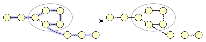
*Figure 4: Augmenting path through a blossom*
Figure 4 shows an augmenting path that runs through a blossom.
The augmenting path runs through an even number of internal edges in the blossom,
which in this case is not the shortest way around the blossom.
After augmenting, the blossom has become reoriented:
a different vertex became the base vertex.
In case of nested blossoms, non-trivial sub-blossoms on the augmenting path must
be updated recursively.
Note that the process of repeatedly augmenting the matching will never cause a matched vertex
to become unmatched.
Once a vertex is matched, augmenting may cause the vertex to become matched to a _different_
vertex, but it can not cause the vertex to become unmatched.
### Edge slack and dual variables
We still need a method to determine which edges are _tight_.
This is done by means of so-called _dual variables_.
The purpose of dual variables can be explained by rephrasing the maximum matching problem
as an instance of linear programming.
I'm not going to do that here.
I will describe how the algorithm uses dual variables without explaining why.
For the mathematical background, I recommend reading [[5]](#galil1986) .
Every vertex _x_ has a dual variable _ux_.
Furthermore, every non-trivial blossom _B_ has a dual variable _zB_.
These variables contain non-negative numbers which change over time through actions
of the algorithm.
Every edge in the graph imposes a constraint on the dual variables:
The weight of the edge between vertices _x_ and _y_ must be less or equal
to the sum of the dual variables _ux_ plus _uy_ plus all
_zB_ of blossoms _B_ that contain the edge.
(A blossom contains an edge if it contains both incident vertices.)
This constraint is more clearly expressed in a formula:
$$ u_x + u_y + \sum_{(x,y) \in B} z_B \ge w_{x,y} $$
The slack _πx,y_ of the edge between vertices _x_ and _y_ is a non-negative number
that indicates how much room is left before the edge constraint would be violated:
$$ \pi_{x,y} = u_x + u_y + \sum_{(x,y) \in B} z_B - w_{x,y} $$
An edge is _tight_ if and only if its slack is zero.
Given the values of the dual variables, it is very easy to calculate the slack of an edge
which is not contained in any blossom: simply add the duals of its incident vertices and
subtract the weight.
To check whether an edge is tight, simply compute its slack and check whether it is zero.
Calculating the slack of an edge that is contained in one or more blossoms is a little tricky,
but fortunately we don't need such calculations.
The search for augmenting paths only considers edges that span _between_ top-level blossoms,
not edges that are contained inside blossoms.
So we never need to check the tightness of internal edges in blossoms.
A matching has maximum weight if it satisfies all of the following constraints:
- All dual variables and edge slacks are non-negative:
_ui_ ≥ 0 , _zB_ ≥ 0 , _πx,y_ ≥ 0
- All matched edges have zero slack: edge _(x, y)_ matched implies _πx,y_ = 0
- All unmatched vertices have dual variable zero: vertex _x_ unmatched implies _ux_ = 0
The first two constraints are satisfied at all times while the matching algorithm runs.
When the algorithm updates dual variables, it ensures that dual variables and edge slacks
remain non-negative.
It also ensures that matched edges remain tight, and that edges which are part of the odd-length
cycle in a blossom remain tight.
When the algorithm augments the matching, it uses an augmenting path that consists of
only tight edges, thus ensuring that newly matched edges have zero slack.
The third constraint is initially not satisfied.
The algorithm makes progress towards satisfying this constraint in two ways:
by augmenting the matching, thus reducing the number of unmatched vertices,
and by reducing the value of the dual variables of unmatched vertices.
Eventually, either all vertices are matched or all unmatched vertices have zero dual.
At that point the maximum weight matching has been found.
When the matching algorithm is finished, the constraints can be checked to verify
that the matching is optimal.
This check is simpler and faster than the matching algorithm itself.
It can therefore be a useful way to guard against bugs in the matching algorithm.
### Rules for updating dual variables
At the start of the matching algorithm, all vertex dual variables _ui_
are initialized to the same value: half of the greatest edge weight value that
occurs on any edge in the graph.
$$ u_i = {1 \over 2} \cdot \max_{(x,y) \in E} w_{x,y} $$
Initially, there are no blossoms yet so there are no _zB_ to be initialized.
When the algorithm creates a new blossom, it initializes its dual variable to
_zB_ = 0.
Note that this does not change the slack of any edge.
If a search for an augmenting path fails while there are still unmatched vertices
with positive dual variables, it may not yet have found the maximum weight matching.
In such cases the algorithm updates the dual variables until either
an augmenting path gets unlocked or the dual variables of all unmatched vertices reach zero.
To update the dual variables, the algorithm chooses a value _δ_ that represents how much
the duals will change.
It then changes dual variables as follows:
- _ux ← ux − δ_ for every S-vertex _x_
- _ux ← ux + δ_ for every T-vertex _x_
- _zB ← zB + 2 * δ_ for every non-trivial S-blossom _B_
- _zB ← zB − 2 * δ_ for every non-trivial T-blossom _B_
Dual variables of unlabeled blossoms and their vertices remain unchanged.
Dual variables _zB_ of non-trivial sub-blossoms also remain changed;
only top-level blossoms have their _zB_ updated.
Note that this update does not change the slack of edges that are either matched,
or linked in the alternating tree, or contained in a blossom.
However, the update reduces the slack of edges between S blossoms and edges between S-blossoms
and unlabeled blossoms.
It may cause some of these edges to become tight, allowing them to be used
to construct an augmenting path.
The value of _δ_ is determined as follows:
_δ_ = min(_δ1_, _δ2_, _δ3_, _δ4_) where
- _δ1_ is the minimum _ux_ of any S-vertex _x_.
- _δ2_ is the minimum slack of any edge between an S-blossom and
an unlabeled blossom.
- _δ3_ is half of the minimum slack of any edge between two different S-blossoms.
- _δ4_ is half of the minimum _zB_ of any T-blossom _B_.
_δ1_ protects against any vertex dual becoming negative.
_δ2_ and _δ3_ together protect against any edge slack
becoming negative.
_δ4_ protects against any blossom dual becoming negative.
If the dual update is limited by _δ1_, it causes the duals of all remaining
unmatched vertices to become zero.
At that point the maximum matching has been found and the algorithm ends.
If the dual update is limited by _δ2_ or _δ3_, it causes
an edge to become tight.
The next step is to either add that edge to the alternating tree (_δ2_)
or use it to construct a blossom or augmenting path (_δ3_).
If the dual update is limited by _δ4_, it causes the dual variable of
a T-blossom to become zero.
The next step is to expand that blossom.
A dual update may find that _δ = 0_, implying that the dual variables don't change.
This can still be useful since all types of updates have side effects (adding an edge
to an alternating tree, or expanding a blossom) that allow the algorithm to make progress.
During a single _stage_, the algorithm may iterate several times between scanning tight edges and
updating dual variables.
These iterations are called _substages_.
To clarify: A stage is the process of growing alternating trees until an augmenting path is found.
A stage ends either by augmenting the matching, or by concluding that no further improvement
is possible.
Each stage consists of one or more substages.
A substage scans tight edges to grow the alternating trees.
When a substage runs out of tight edges, it ends by performing a dual variable update.
A substage also ends immediately when it finds an augmenting path.
At the end of each stage, labels and alternating trees are removed.
The matching algorithm ends when a substage ends in a dual variable update limited
by _δ1_.
At that point the matching has maximum weight.
### Expanding a blossom
There are two scenarios where a blossom must be expanded.
One is when the dual variable of a T-blossom becomes zero after a dual update limited
by _δ4_.
In this case the blossom must be expanded, otherwise further dual updates would cause
its dual to become negative.
The other scenario is when the algorithm is about to assign label T to an unlabeled blossom
with dual variable zero.
A T-blossom with zero dual serves no purpose, potentially blocks an augmenting path,
and is likely to be expanded anyway via a _δ4=0_ update.
It is therefore better to preemptively expand the unlabeled blossom.
The step that would have assigned label T to the blossom is then re-evaluated,
which will cause it to assign label T to a sub-blossom of the expanded blossom.
It may then turn out that this sub-blossom must also be expanded, and this becomes
a recursive process until we get to a sub-blossom that is either a single vertex or
a blossom with non-zero dual.
Note that [[5]](#galil1986) specifies that all top-level blossoms with dual variable zero should be
expanded after augmenting the matching.
This prevents the existence of unlabeled top-level blossoms with zero dual,
and therefore prevents the scenario where label T would be assigned to such blossoms.
That strategy is definitely correct, but it may lead to unnecessary expanding
of blossoms which are then recreated during the search for the next augmenting path.
Postponing the expansion of these blossoms until they are about to be labeled T,
as described above, may be faster in some cases.
Expanding an unlabeled top-level blossom _B_ is pretty straightforward.
Simply promote all of its sub-blossoms to top-level blossoms, then delete _B_.
Note that the slack of all edges remains unchanged, since _zB = 0_.
Expanding a T-blossom is tricky because the labeled blossom is part of an alternating tree.
After expanding the blossom, the part of the alternating tree that runs through the blossom
must be reconstructed.
An alternating path through a blossom always runs through its base vertex.
After expanding T-blossom _B_, we can reconstruct the alternating path by following it
from the sub-blossom where the path enters _B_ to the sub-blossom that contains the base vertex
(choosing the direction around the blossom that takes an even number of steps).
We then assign alternating labels T and S to the sub-blossoms along that path
and link them into the alternating tree.
All vertices of sub-blossoms that got label S are inserted into _Q_.

*Figure 5: Expanding a T-blossom*
### Keeping track of least-slack edges
To perform a dual variable update, the algorithm needs to compute the values
of _δ1_, _δ2_, _δ3_ and _δ4_
and determine which edge (_δ2_, _δ3_) or
blossom (_δ4_) achieves the minimum value.
The total number of dual updates during a matching may be _Θ(n2)_.
Since we want to limit the total number of steps of the matching algorithm to _O(n3)_,
each dual update may use at most _O(n)_ steps.
We can find _δ1_ in _O(n)_ steps by simply looping over all vertices
and checking their dual variables.
We can find _δ4_ in _O(n)_ steps by simply looping over all non-trivial blossoms
(since there are fewer than _n_ non-trivial blossoms).
We could find _δ2_ and _δ3_ by simply looping over
all edges of the graph in _O(m)_ steps, but that exceeds our budget of _O(n)_ steps.
So we need better techniques.
For _δ2_, we determine the least-slack edge between an S-blossom and unlabeled
blossom as follows.
For every vertex _y_ in any unlabeled blossom, keep track of _ey_:
the least-slack edge that connects _y_ to any S-vertex.
The thing to keep track of is the identity of the edge, not the slack value.
This information is kept up-to-date as part of the procedure that considers S-vertices.
The scanning procedure eventually considers all edges _(x, y, w)_ where _x_ is an S-vertex.
At that moment _ey_ is updated if the new edge has lower slack.
Calculating _δ2_ then becomes a matter of looping over all vertices _x_,
checking whether _B(x)_ is unlabeled and calculating the slack of _ex_.
One subtle aspect of this technique is that a T-vertex can loose its label when
the containing T-blossom gets expanded.
At that point, we suddenly need to have kept track of its least-slack edge to any S-vertex.
It is therefore necessary to do the same tracking also for T-vertices.
So the technique is: For any vertex that is not an S-vertex, track its least-slack edge
to any S-vertex.
Another subtle aspect is that a T-vertex may have a zero-slack edge to an S-vertex.
Even though these edges are already tight, they must still be tracked.
If the T-vertex loses its label, this edge needs to be reconsidered by the scanning procedure.
By including these edges in least-slack edge tracking, they will be rediscovered
through a _δ2=0_ update after the vertex becomes unlabeled.
For _δ3_, we determine the least-slack edge between any pair of S-blossoms
as follows.
For every S-blossom _B_, keep track of _eB_:
the least-slack edge between _B_ and any other S-blossom.
Note that this is done per S-blossoms, not per S-vertex.
This information is kept up-to-date as part of the procedure that considers S-vertices.
Calculating _δ3_ then becomes a matter of looping over all S-blossoms _B_
and calculating the slack of _eB_.
A complication occurs when S-blossoms are merged.
Some of the least-slack edges of the sub-blossoms may be internal edges in the merged blossom,
and therefore irrelevant for _δ3_.
As a result, the proper _eB_ of the merged blossom may be different from all
least-slack edges of its sub-blossoms.
An additional data structure is needed to find _eB_ of the merged blossom.
For every S-blossom _B_, maintain a list _LB_ of edges between _B_ and
other S-blossoms.
The purpose of _LB_ is to contain, for every other S-blossom, the least-slack edge
between _B_ and that blossom.
These lists are kept up-to-date as part of the procedure that considers S-vertices.
While considering vertex _x_, if edge _(x, y, w)_ has positive slack,
and _B(y)_ is an S-blossom, the edge is inserted in _LB(x)_.
This may cause _LB(x)_ to contain multiple edges to _B(y)_.
That's okay as long as it definitely contains the least-slack edge to _B(y)_.
When a new S-blossom is created, form its list _LB_ by merging the lists
of its sub-blossoms.
Ignore edges that are internal to the merged blossom.
If there are multiple edges to the same target blossom, keep only the least-slack of these edges.
Then find _eB_ of the merged blossom by simply taking the least-slack edge
out of _LB_.
## Run time of the algorithm
Every stage of the algorithm either increases the number of matched vertices by 2 or
ends the matching.
Therefore the number of stages is at most _n/2_.
Every stage runs in _O(n2)_ steps, therefore the complete algorithm runs in
_O(n3)_ steps.
During each stage, edge scanning is driven by the queue _Q_.
Every vertex enters _Q_ at most once.
Each vertex that enters _Q_ has its incident edges scanned, causing every edge in the graph
to be scanned at most twice per stage.
Scanning an edge is done in constant time, unless it leads to the discovery of a blossom
or an augmenting path, which will be separately accounted for.
Therefore edge scanning needs _O(m)_ steps per stage.
Creating a blossom reduces the number of top-level blossoms by at least 2,
thus limiting the number of simultaneously existing blossoms to _O(n)_.
Blossoms that are created during a stage become S-blossoms and survive until the end of that stage,
therefore _O(n)_ blossoms are created during a stage.
Creating a blossom involves tracing the alternating path to the closest common ancestor,
and some bookkeeping per sub-blossom,
and inserting new S-vertices _Q_,
all of which can be done in _O(n)_ steps per blossom creation.
The cost of managing least-slack edges between S-blossoms will be separately accounted for.
Therefore blossom creation needs _O(n2)_ steps per stage
(excluding least-slack edge management).
As part of creating a blossom, a list _LB_ of least-slack edges must be formed.
This involves processing every element of all least-slack edge lists of its sub-blossoms,
and removing redundant edges from the merged list.
Merging and removing redundant edges can be done in one sweep via a temporary array indexed
by target blossom.
Collect the least-slack edges of the sub-blossoms into this array,
indexed by the target blossom of the edge,
keeping only the edge with lowest slack per target blossom.
Then convert the array back into a list by removing unused indices.
This takes _O(1)_ steps per candidate edge, plus _O(n)_ steps to manage the temporary array.
I choose to shift the cost of collecting the candidate edges from the sub-blossoms to
the actions that inserted those edges into the sub-blossom lists.
There are two processes which insert edges into _LB_: edge scanning and blossom
creation.
Edge scanning inserts each graph edge at most twice per stage for a total cost of _O(m)_ steps
per stage.
Blossom creation inserts at most _O(n)_ edges per blossom creation.
Therefore the total cost of S-blossom least-slack edge management is
_O(m + n2) = O(n2)_ steps per stage.
The number of blossom expansions during a stage is _O(n)_.
Expanding a blossom involves some bookkeeping per sub-blossom,
and reconstructing the alternating path through the blossom,
and inserting any new S-vertices into _Q_,
all of which can be done in _O(n)_ steps per blossom.
Therefore blossom expansion needs _O(n2)_ steps per stage.
The length of an augmenting path is _O(n)_.
Tracing the augmenting path and augmenting the matching along the path can be done in _O(n)_ steps.
Augmenting through a blossom takes a number of steps that is proportional in the number of
its sub-blossoms.
Since there are fewer than _n_ non-trivial blossoms, the total cost of augmenting through
blossoms is _O(n)_ steps.
Therefore the total cost of augmenting is _O(n)_ steps per stage.
A dual variable update limited by _δ1_ ends the algorithm and therefore
happens at most once.
An update limited by _δ2_ labels a previously labeled blossom
and therefore happens _O(n)_ times per stage.
An update limited by _δ3_ either creates a blossom or finds an augmenting path
and therefore happens _O(n)_ times per stage.
An update limited by _δ4_ expands a blossom and therefore happens
_O(n)_ times per stage.
Therefore the number of dual variable updates is _O(n)_ per stage.
The cost of calculating the _δ_ values is _O(n)_ per update as discussed above.
Applying changes to the dual variables can be done by looping over all vertices and looping over
all top-level blossoms in _O(n)_ steps per update.
Therefore the total cost of dual variable updates is _O(n2)_ per stage.
## Implementation details
_TO BE WRITTEN_
## References
1.
Jack Edmonds, "Paths, trees, and flowers." _Canadian Journal of Mathematics vol. 17 no. 3_, 1965.
([link](https://doi.org/10.4153/CJM-1965-045-4))
([pdf](https://www.cambridge.org/core/services/aop-cambridge-core/content/view/08B492B72322C4130AE800C0610E0E21/S0008414X00039419a.pdf/paths_trees_and_flowers.pdf))
2.
Jack Edmonds, "Maximum matching and a polyhedron with 0,1-vertices." _Journal of research of the National Bureau of Standards vol. 69B_, 1965.
([pdf](https://nvlpubs.nist.gov/nistpubs/jres/69B/jresv69Bn1-2p125_A1b.pdf))
3.
Harold N. Gabow, "Implementation of algorithms for maximum matching on nonbipartite graphs." Ph.D. thesis, Stanford University, 1974.
4.
Z. Galil, S. Micali, H. Gabow, "An O(EV log V) algorithm for finding a maximal weighted matching in general graphs." _SIAM Journal on Computing vol. 15 no. 1_, 1986.
([link](https://epubs.siam.org/doi/abs/10.1137/0215009))
([pdf](https://www.researchgate.net/profile/Zvi-Galil/publication/220618201_An_OEVlog_V_Algorithm_for_Finding_a_Maximal_Weighted_Matching_in_General_Graphs/links/56857f5208ae051f9af1e257/An-OEVlog-V-Algorithm-for-Finding-a-Maximal-Weighted-Matching-in-General-Graphs.pdf))
5.
Zvi Galil, "Efficient algorithms for finding maximum matching in graphs." _ACM Computing Surveys vol. 18 no. 1_, 1986.
([link](https://dl.acm.org/doi/abs/10.1145/6462.6502))
([pdf](https://dl.acm.org/doi/pdf/10.1145/6462.6502))
6.
Harold N. Gabow, "Data structures for weighted matching and nearest common ancestors with linking." _Proc. 1st ACM-SIAM symposium on discrete algorithms_, 1990.
([link](https://dl.acm.org/doi/abs/10.5555/320176.320229))
([pdf](https://dl.acm.org/doi/pdf/10.5555/320176.320229))
---
Written in 2023 by Joris van Rantwijk.
This work is licensed under [CC BY-ND 4.0](https://creativecommons.org/licenses/by-nd/4.0/).