# Implementation of Maximum Weighted Matching
## Introduction
This document describes the implementation of an algorithm that computes a maximum weight matching
in a general graph in time _O(n (n + m) log n)_, where _n_ is the number of vertices in
the graph and _m_ is the number of edges.
In graph theory, a _matching_ is a subset of edges such that none of them share a common vertex.
A _maximum cardinality matching_ is a matching that contains the largest possible number of edges
(or equivalently, the largest possible number of vertices).
If a graph has weights assigned to its edges, a _maximum weight matching_
is a matching that achieves the largest possible sum of weights of matched edges.
An algorithm for maximum weight matching can obviously also be used to calculate a maximum
cardinality matching by simply assigning weight 1 to all edges.
Certain related problems can be understood as _restrictions_ of maximum weighted matching
in general graphs.
Examples are: maximum matching in bipartite graphs, maximum cardinality matching in general graphs,
and maximum weighted matching in general graphs with edge weights limited to integers
in a certain range.
Clearly, an algorithm for maximum weighted matching in general graphs also solves
all of these restricted problems.
However, some of the restricted problems can be solved with algorithms that are simpler and/or
faster than the known algorithms for the general problem.
The rest of this document does not consider restricted problems.
My focus is purely on maximum weighted matching in general graphs.
In this document, _n_ refers to the number of vertices and _m_ refers to the number of edges in the graph.
## A timeline of matching algorithms
In 1963, Jack Edmonds published the first polynomial-time algorithm for maximum matching in
general graphs [[1]](#edmonds1965a) [[2]](#edmonds1965b) .
Efficient algorithms for bipartite graphs were already known at the time, but generalizations
to non-bipartite graphs would tend to require an exponential number of steps.
Edmonds solved this by explicitly detecting _blossoms_ (odd-length alternating cycles) and
adding special treatment for them.
He also introduced a linear programming technique to handle weighted matching.
The resulting maximum weighted matching algorithm runs in time _O(n4)_.
In 1973, Harold N. Gabow published a maximum weighted matching algorithm that runs in
time _O(n3)_ [[3]](#gabow1974) .
It is based on the ideas of Edmonds, but uses different data structures to reduce the amount
of work.
In 1983, Galil, Micali and Gabow published a maximum weighted matching algorithm that runs in
time _O(n m log n)_ [[4]](#galil_micali_gabow1986) .
It is an implementation of Edmonds' blossom algorithm that uses advanced data structures
to speed up critical parts of the algorithm.
This algorithm is asymptotically faster than _O(n3)_ for sparse graphs,
but slower for highly dense graphs.
In 1983, Zvi Galil published an overview of algorithms for 4 variants of the matching problem
[[5]](#galil1986) :
maximum-cardinality resp. maximum-weight matching in bipartite resp. general graphs.
I like this paper a lot.
It explains the algorithms from first principles and can be understood without prior knowledge
of the literature.
The paper describes a maximum weighted matching algorithm that is similar to Edmonds'
blossom algorithm, but carefully implemented to run in time _O(n3)_.
It then sketches how advanced data structures can be added to arrive at the Galil-Micali-Gabow
algorithm that runs in time _O(n m log n)_.
In 1990, Gabow published a maximum weighted matching algorithm that runs in time
_O(n m + n2 log n)_ [[6]](#gabow1990) .
It uses several advanced data structures, including Fibonacci heaps.
Unfortunately I don't understand this algorithm at all.
## Choosing an algorithm
I selected the _O(n m log n)_ algorithm by Galil, Micali and Gabow
[[4]](#galil_micali_gabow1986).
This algorithm is asymptotically optimal for sparse graphs.
It has also been shown to be quite fast in practice on several types of graphs
including random graphs [[7]](#mehlhorn_schafer2002).
This algorithm is more difficult to implement than the older _O(n3)_ algorithm.
In particular, it requires a specialized data structure to implement concatenable priority queues.
This increases the size and complexity of the code quite a bit.
However, in my opinion the performance improvement is worth the extra effort.
## Description of the algorithm
My implementation roughly follows the description by Zvi Galil in [[5]](#galil1986) .
I recommend reading that paper before diving into my description below.
The paper explains the algorithm in depth and shows how it relates to matching
in bipartite graphs and non-weighted graphs.
There are subtle aspects to the algorithm that are tricky to implement correctly but are
mentioned only briefly in the paper.
In this section, I describe the algorithm from my own perspective:
a programmer struggling to implement the algorithm correctly.
My goal is only to describe the algorithm, not to prove its correctness.
### Basic concepts
An edge-weighted, undirected graph _G_ consists of a set _V_ of _n_ vertices and a set _E_
of _m_ edges.
Vertices are represented by non-negative integers from _0_ to _n-1_: _V = { 0, 1, ..., n-1 }_
Edges are represented by tuples: _E = { (x, y, w), ... }_
where the edge _(x, y, w)_ is incident on vertices _x_ and _y_ and has weight _w_.
The order of vertices is irrelevant, i.e. _(x, y, w)_ and _(y, x, w)_ represent the same edge.
Edge weights may be integers or floating point numbers.
There can be at most one edge between any pair of vertices.
A vertex can not have an edge to itself.
A matching is a subset of edges without any pair of edges sharing a common vertex.
An edge is matched if it is part of the matching, otherwise it is unmatched.
A vertex is matched if it is incident to an edge in the matching, otherwise it is unmatched.
An alternating path is a simple path that alternates between matched and unmatched edges.
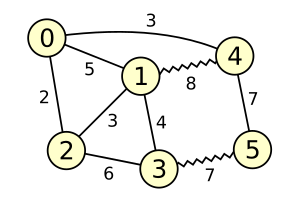
*Figure 1*
Figure 1 depicts a graph with 6 vertices and 9 edges.
Wavy lines represent matched edges; straight lines represent edges that are currently unmatched.
The matching has weight 8 + 7 = 15.
An example of an alternating path would be 0 - 1 - 4 - 5 - 3 (but there are many others).
### Augmenting paths
An augmenting path is an alternating path that begins and ends in two unmatched vertices.
An augmenting path can be used to extend the matching as follows:
remove all matched edges on the augmenting path from the matching,
and add all previously unmatched edges on the augmenting path to the matching.
The result is again a valid matching, and the number of matched edges has increased by one.
The matching in figure 1 above has several augmenting paths.
For example, the edge from vertex 0 to vertex 2 is by itself an augmenting path.
Augmenting along this path would increase the weight of the matching by 2.
Another augmenting path is 0 - 1 - 4 - 5 - 3 - 2, which would increase the weight of
the matching by 3.
Finally, 0 - 4 - 1 - 2 is also an augmenting path, but it would decrease the weight
of the matching by 2.
### Main algorithm
Our algorithm to compute a maximum weighted matching is as follows:
- Start with an empty matching (all edges unmatched).
- Repeat the following steps:
- Find an augmenting path that provides the largest possible increase of the weight of
the matching.
- If there is no augmenting path that increases the weight of the matching,
end the algorithm.
The current matching is a maximum-weight matching.
- Otherwise, use the augmenting path to update the matching.
- Continue by searching for another augmenting path, etc.
This algorithm ends when there are no more augmenting paths that increase the weight
of the matching.
In some cases, there may still be augmenting paths which do not increase the weight of the matching,
implying that the maximum-weight matching has fewer edges than the maximum cardinality matching.
Every iteration of the main loop is called a _stage_.
Note that the final matching contains at most _n/2_ edges, therefore the algorithm
performs at most _n/2_ stages.
The only remaining challenge is finding an augmenting path.
Specifically, finding an augmenting path that increases the weight of the matching
as much as possible.
### Blossoms
A blossom is an odd-length cycle that alternates between matched and unmatched edges.
Such cycles complicate the search for augmenting paths.
To overcome these problems, blossoms must be treated specially.
The trick is to temporarily replace the vertices and edges that are part of the blossom
by a single super-vertex.
This is called _shrinking_ the blossom.
The search for an augmenting path then continues in the modified graph in which
the odd-length cycle no longer exists.
It may later become necessary to _expand_ the blossom (undo the shrinking step).
For example, the cycle 0 - 1 - 4 - 0 in figure 1 above is an odd-length alternating cycle,
and therefore a candidate to become a blossom.
In practice, we do not remove vertices or edges from the graph while shrinking a blossom.
Instead the graph is left unchanged, but a separate data structure keeps track of blossoms
and which vertices are contained in which blossoms.
A graph can contain many blossoms.
Furthermore, after shrinking a blossom, that blossom can become a sub-blossom
in a bigger blossom.
Figure 2 depicts a graph with several nested blossoms.
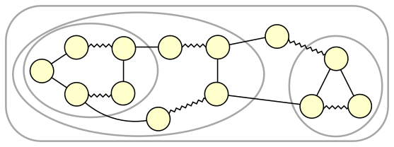
*Figure 2: Nested blossoms*
To describe the algorithm unambiguously, we need precise definitions:
* A _blossom_ is either a single vertex, or an odd-length alternating cycle of _sub-blossoms_.
* A _non-trivial blossom_ is a blossom that is not a single vertex.
* A _top-level blossom_ is a blossom that is not contained inside another blossom.
It can also be a single vertex which is not part of any blossom.
* The _base vertex_ of a blossom is the only vertex in the blossom that is not matched
to another vertex in the same blossom.
The base vertex is either unmatched, or matched to a vertex outside the blossom.
In a single-vertex blossom, its only vertex is the base vertex.
In a non-trivial blossom, the base vertex is equal to the base vertex of the unique sub-blossom
that begins and ends the alternating cycle.
* The _parent_ of a non-top-level blossom is the directly enclosing blossom in which
it occurs as a sub-blossom.
Top-level blossoms do not have parents.
Non-trivial blossoms are created by shrinking and destroyed by expanding.
These are explicit steps of the algorithm.
This implies that _not_ every odd-length alternating cycle is a blossom.
The algorithm decides which cycles are blossoms.
Just before a new blossom is created, its sub-blossoms are initially top-level blossoms.
After creating the blossom, the sub-blossoms are no longer top-level blossoms because they are contained inside the new blossom, which is now a top-level blossom.
Every vertex is contained in precisely one top-level blossom.
This may be either a trivial blossom which contains only that single vertex,
or a non-trivial blossom into which the vertex has been absorbed through shrinking.
A vertex may belong to different top-level blossoms over time as blossoms are
created and destroyed by the algorithm.
I use the notation _B(x)_ to indicate the top-level blossom that contains vertex _x_.
### Searching for an augmenting path
Recall that the matching algorithm repeatedly searches for an augmenting path that
increases the weight of the matching as much as possible.
I'm going to postpone the part that deals with "increasing the weight as much as possible".
For now, all we need to know is this:
At a given step in the algorithm, some edges in the graph are _tight_ while other edges
have _slack_.
An augmenting path that consists only of tight edges is _guaranteed_ to increase the weight
of the matching as much as possible.
While searching for an augmenting path, we restrict the search to tight edges,
ignoring all edges that have slack.
Certain explicit actions of the algorithm cause edges to become tight or slack.
How this works will be explained later.
To find an augmenting path, the algorithm searches for alternating paths that start
in an unmatched vertex.
The collection of such alternating paths forms a forest of trees.
Each tree is rooted in an unmatched vertex, and all paths from the root to the leaves of a tree
are alternating paths.
The nodes in these trees are top-level blossoms.
To facilitate the search, top-level blossoms are labeled as either _S_ or _T_ or _unlabeled_.
Label S is assigned to the roots of the alternating trees, and to nodes at even distance
from the root.
Label T is assigned to nodes at odd distance from the root of an alternating tree.
Unlabeled blossoms are not (yet) part of an alternating tree.
(In some papers, the label S is called _outer_ and T is called _inner_.)
It is important to understand that labels S and T are assigned only to top-level blossoms,
not to individual vertices.
However, it is often relevant to know the label of the top-level blossom that contains
a given vertex.
I use the following terms for convenience:
* an _S-blossom_ is a top-level blossom with label S;
* a _T-blossom_ is a top-level blossom with label T;
* an _S-vertex_ is a vertex inside an S-blossom;
* a _T-vertex_ is a vertex inside a T-blossom.
Edges that span between two S-blossoms are special.
If both S-blossoms are part of the same alternating tree, the edge is part of
an odd-length alternating cycle.
The lowest common ancestor node in the alternating tree forms the beginning and end
of the alternating cycle.
In this case a new blossom must be created by shrinking the cycle.
On the other hand, if the two S-blossoms are in different alternating trees,
the edge that links the blossoms is part of an augmenting path between the roots of the two trees.
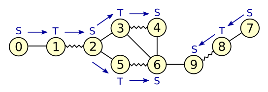
*Figure 3: Growing alternating trees*
The graph in figure 3 contains two unmatched vertices: 0 and 7.
Both form the root of an alternating tree.
Blue arrows indicate edges in the alternating trees, pointing away from the root.
The graph edge between vertices 4 and 6 connects two S-blossoms in the same alternating tree.
Scanning this edge will cause the creation of a new blossom with base vertex 2.
The graph edge between vertices 6 and 9 connects two S-blossoms which are part
of different alternating trees.
Scanning this edge will discover an augmenting path between vertices 0 and 7.
Note that all vertices in the graph of figure 3 happen to be top-level blossoms.
In general, the graph may already contain non-trivial blossoms.
Alternating trees are constructed over top-level blossoms, not necessarily over
individual vertices.
When a vertex becomes an S-vertex, it is added to a queue.
The search procedure considers these vertices one-by-one and tries to use them to
either grow the alternating tree (thus adding new vertices to the queue),
or discover an augmenting path or a new blossom.
The search for an augmenting path proceeds as follows:
- Mark all top-level blossoms as _unlabeled_.
- Initialize an empty queue _Q_.
- Assign label S to all top-level blossoms that contain an unmatched vertex.
Add all vertices inside such blossoms to _Q_.
- Repeat until _Q_ is empty:
- Take a vertex _x_ from _Q_.
- Scan all _tight_ edges _(x, y, w)_ that are incident on vertex _x_.
- Find the top-level blossom _B(x)_ that contains vertex _x_
and the top-level blossom _B(y)_ that contains vertex _y_.
- If _B(x)_ and _B(y)_ are the same blossom, ignore this edge.
(It is an internal edge in the blossom.)
- Otherwise, if blossom _B(y)_ is unlabeled, assign label T to it.
The base vertex of _B(y)_ is matched (otherwise _B(y)_ would have label S).
Find the vertex _t_ which is matched to the base vertex of _B(y)_ and find
its top-level blossom _B(t)_ (this blossom is still unlabeled).
Assign label S to blossom _B(t)_, and add all vertices inside _B(t)_ to _Q_.
- Otherwise, if blossom _B(y)_ has label T, ignore this edge.
- Otherwise, if blossom _B(y)_ has label S, there are two scenarios:
- Either _B(x)_ and _B(y)_ are part of the same alternating tree.
In that case, we have discovered an odd-length alternating cycle.
Shrink the cycle into a blossom and assign label S to it.
Add all vertices inside its T-labeled sub-blossoms to _Q_.
(Vertices inside S-labeled sub-blossoms have already been added to _Q_
and must not be added again.)
Continue the search for an augmenting path.
- Otherwise, if _B(x)_ and _B(y)_ are part of different alternating trees,
we have found an augmenting path between the roots of those trees.
End the search and return the augmenting path.
- If _Q_ becomes empty before an augmenting path has been found,
it means that no augmenting path exists (which consists of only tight edges).
For each top-level blossom, we keep track of its label as well as the edge through
which it obtained its label (attaching it to the alternating tree).
These edges are needed to trace back through the alternating tree to construct
a blossom or an alternating path.
When an edge between S-blossoms is discovered, it is handled as follows:
- The two top-level blossoms are _B(x)_ and _B(y)_, both labeled S.
- Trace up through the alternating trees from _B(x)_ and _B(y)_ towards the root.
- If the blossoms are part of the same alternating tree, the tracing process
eventually reaches a lowest common ancestor of _B(x)_ and _B(y)_.
In that case a new blossom must be created.
Its alternating cycle starts at the common ancestor, follows the path through
the alternating tree down to _B(x)_, then via the scanned edge to _B(y)_,
then through the alternating tree up to the common ancestor.
(Note it is possible that either _B(x)_ or _B(y)_ is itself the lowest common ancestor.)
- Otherwise, the blossoms are in different trees.
The tracing process will eventually reach the roots of both trees.
At that point we have traced out an augmenting path between the two roots.
Note that the matching algorithm uses two different types of tree data structures.
These two types of trees are separate concepts.
But since they are both trees, there is potential for accidentally confusing them.
It may be helpful to explicitly distinguish the two types:
- A forest of _blossom structure trees_ represents the nested structure of blossoms.
Every node in these trees is a blossom.
The roots are the top-level blossoms.
The leaf nodes are the single vertices.
The child nodes of each non-leaf node represent its sub-blossoms.
Every vertex is a leaf node in precisely one blossom structure tree.
A blossom structure tree may consist of just one single node, representing
a vertex that is not part of any non-trivial blossom.
- A forest of _alternating trees_ represents an intermediate state during the search
for an augmenting path.
Every node in these trees is a top-level blossom.
The roots are top-level blossoms with an unmatched base vertex.
Every labeled top-level blossom is part of an alternating tree.
Unlabeled blossoms are not (yet) part of a tree.
### Augmenting the matching
Once an augmenting path has been found, augmenting the matching is relatively easy.
Simply follow the path, adding previously unmatched edges to the matching and removing
previously matched edges from the matching.
A useful data structure to keep track of matched edges is an array `mate[x]` indexed by vertex.
If vertex _x_ is matched, `mate[x]` contains the index of the vertex to which it is matched.
If vertex _x_ is unmatched, `mate[x]` contains -1.
A slight complication arises when the augmenting path contains a non-trivial blossom.
The search returns an augmenting path over top-level blossoms, without details
about the layout of the path within blossoms.
Any parts of the path that run through a blossom must be traced in order to update
the matched/unmatched status of the edges in the blossom.
When an augmenting path runs through a blossom, it always runs between the base vertex of
the blossom and some sub-blossom (potentially the same sub-blossom that contains the base vertex).
If the base vertex is unmatched, it forms the start or end of the augmenting path.
Otherwise, the augmenting path enters the blossom though the matched edge of the base vertex.
From the opposite direction, the augmenting path enters the blossom through an unmatched edge.
It follows that the augmenting path must run through an even number of internal edges
of the blossom.
Fortunately, every sub-blossom can be reached from the base through an even number of steps
by walking around the blossom in the appropriate direction.
Augmenting along a path through a blossom causes a reorientation of the blossom.
Afterwards, it is still a blossom and still consists of an odd-length alternating cycle,
but the cycle begins and ends in a different sub-blossom.
The blossom also has a different base vertex.
(In specific cases where the augmenting path merely "grazes" a blossom,
the orientation and base vertex remain unchanged.)
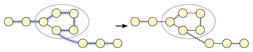
*Figure 4: Augmenting path through a blossom*
Figure 4 shows an augmenting path that runs through a blossom.
The augmenting path runs through an even number of internal edges in the blossom,
which in this case is not the shortest way around the blossom.
After augmenting, the blossom has become reoriented:
a different vertex became the base vertex.
In case of nested blossoms, non-trivial sub-blossoms on the augmenting path must
be updated recursively.
Note that the process of repeatedly augmenting the matching will never cause a matched vertex
to become unmatched.
Once a vertex is matched, augmenting may cause the vertex to become matched to a _different_
vertex, but it can not cause the vertex to become unmatched.
### Edge slack and dual variables
We still need a method to determine which edges are _tight_.
This is done by means of so-called _dual variables_.
The purpose of dual variables can be explained by rephrasing the maximum matching problem
as an instance of linear programming.
I'm not going to do that here.
I will describe how the algorithm uses dual variables without explaining why.
For the mathematical background, I recommend reading [[5]](#galil1986) .
Every vertex _x_ has a dual variable _ux_.
Furthermore, every non-trivial blossom _B_ has a dual variable _zB_.
These variables contain non-negative numbers which change over time through actions
of the algorithm.
Every edge in the graph imposes a constraint on the dual variables:
The weight of the edge between vertices _x_ and _y_ must be less or equal
to the sum of the dual variables _ux_ plus _uy_ plus all
_zB_ of blossoms _B_ that contain the edge.
(A blossom contains an edge if it contains both incident vertices.)
This constraint is more clearly expressed in a formula:
$$ u_x + u_y + \sum_{(x,y) \in B} z_B \ge w_{x,y} $$
The slack _πx,y_ of the edge between vertices _x_ and _y_ is a non-negative number
that indicates how much room is left before the edge constraint would be violated:
$$ \pi_{x,y} = u_x + u_y + \sum_{(x,y) \in B} z_B - w_{x,y} $$
An edge is _tight_ if and only if its slack is zero.
Given the values of the dual variables, it is very easy to calculate the slack of an edge
which is not contained in any blossom: add the duals of its incident vertices and
subtract the weight.
To check whether an edge is tight, simply compute its slack and compare it to zero.
Calculating the slack of an edge that is contained in one or more blossoms is a little tricky,
but fortunately we don't need such calculations.
The search for augmenting paths only considers edges that span _between_ top-level blossoms,
not edges that are contained inside blossoms.
So we never need to check the tightness of internal edges in blossoms.
A matching has maximum weight if it satisfies all of the following constraints:
- All dual variables and edge slacks are non-negative:
_ui_ ≥ 0 , _zB_ ≥ 0 , _πx,y_ ≥ 0
- All matched edges have zero slack: edge _(x, y)_ matched implies _πx,y_ = 0
- All unmatched vertices have dual variable zero: vertex _x_ unmatched implies _ux_ = 0
The first two constraints are satisfied at all times while the matching algorithm runs.
When the algorithm updates dual variables, it ensures that dual variables and edge slacks
remain non-negative.
It also ensures that matched edges remain tight, and that edges which are part of the odd-length
cycle in a blossom remain tight.
When the algorithm augments the matching, it uses an augmenting path that consists of
only tight edges, thus ensuring that newly matched edges have zero slack.
The third constraint is initially not satisfied.
The algorithm makes progress towards satisfying this constraint in two ways:
by augmenting the matching, thus reducing the number of unmatched vertices,
and by reducing the value of the dual variables of unmatched vertices.
Eventually, either all vertices are matched or all unmatched vertices have zero dual.
At that point the maximum weight matching has been found.
When the matching algorithm is finished, the constraints can be checked to verify
that the matching is optimal.
This check is simpler and faster than the matching algorithm itself.
It can therefore be a useful way to guard against bugs in the algorithm.
### Rules for updating dual variables
At the start of the matching algorithm, all vertex dual variables _ui_
are initialized to the same value: half of the greatest edge weight value that
occurs on any edge in the graph.
$$ u_i = {1 \over 2} \cdot \max_{(x,y) \in E} w_{x,y} $$
Initially, there are no blossoms yet so there are no _zB_ to be initialized.
When the algorithm creates a new blossom, it initializes its dual variable to
_zB_ = 0.
Note that this does not change the slack of any edge.
If a search for an augmenting path fails while there are still unmatched vertices
with positive dual variables, it may not yet have found the maximum weight matching.
In such cases the algorithm updates the dual variables until either
an augmenting path gets unlocked or the dual variables of all unmatched vertices reach zero.
To update the dual variables, the algorithm chooses a value _δ_ that represents how much
the duals will change.
It then changes dual variables as follows:
- _ux ← ux − δ_ for every S-vertex _x_
- _ux ← ux + δ_ for every T-vertex _x_
- _zB ← zB + 2 * δ_ for every non-trivial S-blossom _B_
- _zB ← zB − 2 * δ_ for every non-trivial T-blossom _B_
Dual variables of unlabeled blossoms and their vertices remain unchanged.
Dual variables _zB_ of non-trivial sub-blossoms also remain unchanged;
only top-level blossoms have their _zB_ updated.
Note that these rules ensure that no change occurs to the slack of any edge which is matched,
or part of an alternating tree, or contained in a blossom.
Such edges are tight and remain tight through the update.
However, the update reduces the slack of edges between S blossoms and edges between S-blossoms
and unlabeled blossoms.
It may cause some of these edges to become tight, allowing them to be used
to construct an augmenting path.
The value of _δ_ is determined as follows:
_δ_ = min(_δ1_, _δ2_, _δ3_, _δ4_) where
- _δ1_ is the minimum _ux_ of any S-vertex _x_.
- _δ2_ is the minimum slack of any edge between an S-blossom and
an unlabeled blossom.
- _δ3_ is half of the minimum slack of any edge between two different S-blossoms.
- _δ4_ is half of the minimum _zB_ of any T-blossom _B_.
_δ1_ protects against any vertex dual becoming negative.
_δ2_ and _δ3_ together protect against any edge slack
becoming negative.
_δ4_ protects against any blossom dual becoming negative.
If the dual update is limited by _δ1_, it causes the duals of all remaining
unmatched vertices to become zero.
At that point the maximum matching has been found and the algorithm ends.
If the dual update is limited by _δ2_ or _δ3_, it causes
an edge to become tight.
The next step is to either add that edge to the alternating tree (_δ2_)
or use it to construct a blossom or augmenting path (_δ3_).
If the dual update is limited by _δ4_, it causes the dual variable of
a T-blossom to become zero.
The next step is to expand that blossom.
### Discovering tight edges through delta steps
A delta step may find that _δ = 0_, implying that the dual variables don't change.
This can still be useful since all types of updates have side effects (adding an edge
to an alternating tree, or expanding a blossom) that allow the algorithm to make progress.
In fact, it is convenient to let the dual update mechanism drive the entire process of discovering
tight edges and growing alternating trees.
In my description of the search algorithm above, I stated that upon discovery of a tight edge
between a newly labeled S-vertex and an unlabeled vertex or a different S-blossom, the edge should
be used to grow the alternating tree or to create a new blossom or to form an augmenting path.
However, it turns out to be easier to postpone the use of such edges until the next delta step.
While scanning newly labeled S-vertices, edges to unlabeled vertices or different S-blossoms
are discovered but not yet used.
Such edges are merely registered in a suitable data structure.
Even if the edge is tight, it is registered rather than used right away.
Once the scan completes, a delta step will be done.
If any tight edges were discovered during the scan, the delta step will find that either
_δ2 = 0_ or _δ3 = 0_.
The corresponding step (growing the alternating tree, creating a blossom or augmenting
the matching) will occur at that point.
If no suitable tight edges exist, a real (non-zero) change of dual variables will occur.
The search for an augmenting path becomes as follows:
- Mark all top-level blossoms as _unlabeled_.
- Initialize an empty queue _Q_.
- Assign label S to all top-level blossoms that contain an unmatched vertex.
Add all vertices inside such blossoms to _Q_.
- Repeat until either an augmenting path is found or _δ1 = 0_:
- Scan all vertices in Q as described earlier.
Register edges to unlabeled vertices or other S-blossoms.
Do not yet use such edges to change the alternating tree, even if the edge is tight.
- Calculate _δ_ and update dual variables as described above.
- If _δ = δ1_, end the search.
The maximum weight matching has been found.
- If _δ = δ2_, use the corresponding edge to grow the alternating tree.
Assign label T to the unlabeled blossom.
Then assign label S to its mate and add the new S-vertices to _Q_.
- If _δ = δ3_ and the corresponding edge connects two S-blossoms
in the same alternating tree, use the edge to create a new blossom.
Add the new S-vertices to _Q_.
- If _δ = δ3_ and the corresponding edge connects two S-blossoms
in different alternating trees, use the edge to construct an augmenting path.
End the search and return the augmenting path.
- If _δ = δ4_, expand the corresponding T-blossom.
It may seem complicated, but this is actually easier.
The code that scans newly labeled S-vertices, no longer needs special treatment of tight edges.
In general, multiple updates of the dual variables are necessary during a single _stage_ of
the algorithm.
Remember that a stage is the process of growing alternating trees until an augmenting path is found.
A stage ends either by augmenting the matching, or by concluding that no further improvement
is possible.
### Expanding a blossom
There are two scenarios where a blossom must be expanded.
One is when the dual variable of a T-blossom becomes zero after a dual update limited
by _δ4_.
In this case the blossom must be expanded, otherwise further dual updates would cause
its dual to become negative.
The other scenario is when the algorithm is about to assign label T to an unlabeled blossom
with dual variable zero.
A T-blossom with zero dual serves no purpose, potentially blocks an augmenting path,
and is likely to be expanded anyway via a _δ4=0_ update.
It is therefore better to preemptively expand the unlabeled blossom.
The step that would have assigned label T to the blossom is then re-evaluated,
which will cause it to assign label T to a sub-blossom of the expanded blossom.
It may then turn out that this sub-blossom must also be expanded, and this becomes
a recursive process until we get to a sub-blossom that is either a single vertex or
a blossom with non-zero dual.
Note that [[5]](#galil1986) specifies that all top-level blossoms with dual variable zero should be
expanded after augmenting the matching.
This prevents the existence of unlabeled top-level blossoms with zero dual,
and therefore prevents the scenario where label T would be assigned to such blossoms.
That strategy is definitely correct, but it may lead to unnecessary expanding
of blossoms which are then recreated during the search for the next augmenting path.
Postponing the expansion of these blossoms until they are about to be labeled T,
as described above, may be faster in some cases.
Expanding an unlabeled top-level blossom _B_ is pretty straightforward.
Simply promote all of its sub-blossoms to top-level blossoms, then delete _B_.
Note that the slack of all edges remains unchanged, since _zB = 0_.
Expanding a T-blossom is tricky because the labeled blossom is part of an alternating tree.
After expanding the blossom, the part of the alternating tree that runs through the blossom
must be reconstructed.
An alternating path through a blossom always runs through its base vertex.
After expanding T-blossom _B_, we can reconstruct the alternating path by following it
from the sub-blossom where the path enters _B_ to the sub-blossom that contains the base vertex
(choosing the direction around the blossom that takes an even number of steps).
We then assign alternating labels T and S to the sub-blossoms along that path
and link them into the alternating tree.
All vertices of sub-blossoms that got label S are inserted into _Q_.
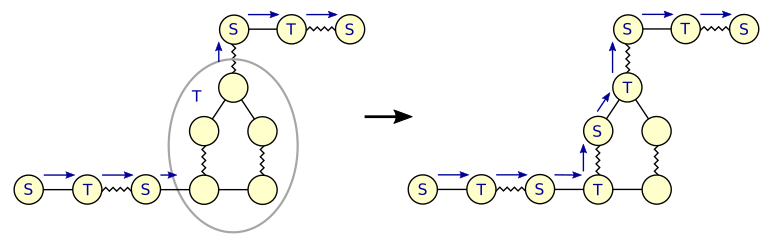
*Figure 5: Expanding a T-blossom*
### Keeping track of the top-level blossom of each vertex
The algorithm often needs to find the top-level blossom _B(x)_ that contains a given vertex _x_.
A naive implementation may keep this information in an array where the element with
index _x_ holds a pointer to blossom _B(x)_.
Lookup in this array would be fast, but keeping the array up-to-date takes too much time.
There can be _O(n)_ stages, and _O(n)_ blossoms can be created or expanded during a stage,
and a blossom can contain _O(n)_ vertices,
therefore the total number of updates to the array could add up to _O(n3)_.
To solve this, we use a special data structure: a _concatenable priority queue_.
Each top-level blossom maintains an instance of this type of queue, containing its vertices.
Each vertex is a member in precisely one such queue.
To find the top-level blossom _B(x)_ that contains a given vertex _x_, we determine
the queue instance in which the vertex is a member.
This takes time _O(log n)_.
The queue instance corresponds directly to a specific blossom, which we can find
for example by storing a pointer to the blossom inside the queue instance.
When a new blossom is created, the concatenable queues of its sub-blossoms are merged
to form one concatenable queue for the new blossom.
The merged queue contains all vertices of the original queues.
Merging a pair of queues takes time _O(log n)_.
To merge the queues of _k_ sub-blossoms, the concatenation step is repeated _k-1_ times,
taking total time _O(k log n)_.
When a blossom is expanded, its concatenable queue is un-concatenated to recover separate queues
for the sub-blossoms.
This also takes time _O(log n)_ for each sub-blossom.
Implementation details of concatenable queues are discussed later in this document.
### Lazy updating of dual variables
During a delta step, the dual variables of labeled vertices and blossoms change as described above.
Updating these variables directly would take time _O(n)_ per delta step.
The total number of delta steps during a matching may be _Θ(n2)_,
pushing the total time to update dual variables to _O(n3)_ which is too slow.
To solve this, [[4]](#galil_micali_gabow1986) describes a technique that stores dual values
in a _modified_ form which is invariant under delta steps.
The modified values can be converted back to the true dual values when necessary.
[[7]](#mehlhorn_schafer2002) describes a slightly different technique which I find easier
to understand.
My implementation is very similar to theirs.
The first trick is to keep track of the running sum of _δ_ values since the beginning of the algorithm.
Let's call that number _Δ_.
At the start of the algorithm _Δ = 0_, but the value increases as the algorithm goes through delta steps.
For each non-trivial blossom, rather than storing its true dual value, we store a _modified_ dual value:
- For an S-blossom, the modified dual value is _z'B = zB - 2 Δ_
- For a T-blossom, the modified dual value is _z'B = zB + 2 Δ_
- For an unlabeled blossom or non-top-level blossom, the modified dual value is equal
to the true dual value.
These modified values are invariant under delta steps.
Thus, there is no need to update the stored values during a delta step.
Since the modified blossom dual value depends on the label (S or T) of the blossom,
the modified value must be updated whenever the label of the blossom changes.
This update can be done in constant time, and changing the label of a blossom is
in any case an explicit step, so this won't increase the asymptotic run time.
For each vertex, rather than storing its true dual value, we store a _modified_ dual value:
- For an S-vertex, the modified dual value is _u'x = ux + Δ_
- For a T-vertex, the modified dual value is _u'x = ux - offsetB(x) - Δ_
- For an unlabeled vertex, the modified dual value is _u'x = ux - offsetB(x)_
where _offsetB_ is an extra variable which is maintained for each top-level blossom.
Again, the modified values are invariant under delta steps, which implies that no update
to the stored values is necessary during a delta step.
Since the modified vertex dual value depends on the label (S or T) of its top-level blossom,
an update is necessary when that label changes.
For S-vertices, we can afford to apply that update directly to the vertices involved.
This is possible since a vertex becomes an S-vertex at most once per stage.
The situation is more complicated for T-vertices.
During a stage, a T-vertex can become unlabeled if it is part of a T-blossom that gets expanded.
The same vertex can again become a T-vertex, then again become unlabeled during a subsequent
blossom expansion.
In this way, a vertex can transition between T-vertex and unlabeled vertex up to _O(n)_ times
within a stage.
We can not afford to update the stored modified vertex dual so many times.
This is where the _offset_ variables come in.
If a blossom becomes a T-blossom, rather than updating the modified duals of all vertices,
we update only the _offset_ variable of the blossom such that the modified vertex duals
remain unchanged.
If a blossom is expanded, we push the _offset_ values down to its sub-blossoms.
### Efficiently computing _δ_
To perform a delta step, the algorithm computes the values
of _δ1_, _δ2_, _δ3_ and _δ4_
and determines which edge (_δ2_, _δ3_) or
blossom (_δ4_) achieves the minimum value.
A naive implementation might compute _δ_ by looping over the vertices, blossoms and edges
in the graph.
The total number of delta steps during a matching may be _Θ(n2)_,
pushing the total time for _δ_ calculations to _O(n2 m)_ which is much too slow.
[[4]](#galil_micali_gabow1986) introduces a combination of data structures from which
the value of _δ_ can be computed efficiently.
_δ1_ is the minimum dual value of any S-vertex.
This value can be computed in constant time.
The dual value of an unmatched vertex is reduced by _δ_ during every delta step.
Since all vertex duals start with the same dual value _ustart_,
all unmatched vertices have dual value _δ1 = ustart - Δ_.
_δ3_ is half of the minimum slack of any edge between two different S-blossoms.
To compute this efficiently, we keep edges between S-blossoms in a priority queue.
The edges are inserted into the queue during scanning of newly labeled S-vertices.
To compute _δ3_, we simply find the minimum-priority element of the queue.
A complication may occur when a new blossom is created.
Edges that connect different top-level S-blossoms before creation of the new blossom,
may end up as internal edges inside the newly created blossom.
This implies that such edges would have to be removed from the _δ3_ priority queue,
but that would be quite difficult.
Instead, we just let those edges stay in the queue.
When computing the value of _δ3_, we thus have to check whether the minimum
element represents an edge between different top-level blossoms.
If not, we discard such stale elements until we find an edge that does.
A complication occurs when dual variables are updated.
At that point, the slack of any edge between different S-blossoms decreases by _2\*δ_.
But we can not afford to update the priorities of all elements in the queue.
To solve this, we set the priority of each edge to its _modified slack_.
The _modified slack_ of an edge is defined as follows:
$$ \pi'_{x,y} = u'_x + u'_y - w_{x,y} $$
The modified slack is computed in the same way as true slack, except it uses
the modified vertex duals instead of true vertex duals.
Blossom duals are ignored since we will never compute the modified slack of an edge that
is contained inside a blossom.
Because modified vertex duals are invariant under delta steps, so is the modified edge slack.
As a result, the priorities of edges in the priority queue remain unchanged during a delta step.
_δ4_ is half of the minimum dual variable of any T-blossom.
To compute this efficiently, we keep non-trivial T-blossoms in a priority queue.
The blossoms are inserted into the queue when they become a T-blossom and removed from
the queue when they stop being a T-blossom.
A complication occurs when dual variables are updated.
At that point, the dual variable of any T-blossom decreases by _2\*δ_.
But we can not afford to update the priorities of all elements in the queue.
To solve this, we set the priority of each blossom to its _modified_ dual value
_z'B = zB + 2\*Δ_.
These values are invariant under delta steps.
_δ2_ is the minimum slack of any edge between an S-vertex and unlabeled vertex.
To compute this efficiently, we use a fairly complicated strategy that involves
three levels of priority queues.
At the lowest level, every T-vertex or unlabeled vertex maintains a separate priority queue
of edges between itself and any S-vertex.
Edges are inserted into this queue during scanning of newly labeled S-vertices.
Note that S-vertices do not maintain this type of queue.
The priorities of edges in these queues are set to their _modified slack_.
This ensures that the priorities remain unchanged during delta steps.
The priorities also remain unchanged when the T-vertex becomes unlabeled or the unlabeled
vertex becomes a T-vertex.
At the middle level, every T-blossom or unlabeled top-level blossom maintains a priority queue
containing its vertices.
This is in fact the _concatenable priority queue_ that is maintained by every top-level blossom
as was described earlier in this document.
The priority of each vertex in the mid-level queue is set to the minimum priority of any edge
in the low-level queue of that vertex.
If edges are added to (or removed from) the low-level queue, the priority of the corresponding
vertex in the mid-level queue may change.
If the low-level queue of a vertex is empty, that vertex has priority _Infinity_
in the mid-level queue.
At the highest level, unlabeled top-level blossoms are tracked in one global priority queue.
The priority of each blossom in this queue is set to the minimum slack of any edge
from that blossom to an S-vertex plus _Δ_.
These priorities are invariant under delta steps.
To compute _δ2_, we find the minimum priority in the high-level queue
and adjust it by _Δ_.
To find the edge associated with _δ2_,
we use the high-level queue to find the unlabeled blossom with minimum priority,
then use that blossom's mid-level queue to find the vertex with minimum priority,
then use that vertex's low-level queue to find the edge with minimum priority.
The whole thing is a bit tricky, but it works.
### Re-using alternating trees
According to [[5]](#galil1986), labels and alternating trees should be erased at the end of each stage.
However, the algorithm can be optimized by keeping some of the labels and re-using them
in the next stage.
The optimized algorithm erases _only_ the two alternating trees that are part of
the augmenting path.
All blossoms in those two trees lose their labels and become free blossoms again.
Other alternating trees, which are not involved in the augmenting path, are preserved
into the next stage, and so are the labels on the blossoms in those trees.
This optimization is well known and is described for example in [[7]](#mehlhorn_schafer2002).
It does not affect the worst-case asymptotic run time of the algorithm,
but it provides a significant practical speed up for many types of graphs.
Erasing alternating trees is easy enough, but selectively stripping labels off blossoms
has a few implications.
The blossoms that lose their labels need to have their modified dual values updated.
The T-blossoms additionally need to have their _offsetB_ variables updated
to keep the vertex dual values consistent.
For S-blossoms that lose their labels, the modified vertex dual variables are updated directly.
The various priority queues also need updating.
Former T-blossoms must be removed from the priority queue for _δ4_.
Edges incident on former S-vertices must be removed from the priority queues for _δ3_ and _δ2_.
Finally, S-vertices that become unlabeled need to construct a proper priority queue
of incident edges to other S-vertices for _δ2_ tracking.
This involves visiting every incident edge of every vertex in each S-blossom that loses its label.
## Run time of the algorithm
Every stage of the algorithm either increases the number of matched vertices by 2 or
ends the matching.
Therefore the number of stages is at most _n/2_.
Every stage runs in time _O((n + m) log n)_, therefore the complete algorithm runs in
time _O(n (n + m) log n)_.
Creating a blossom reduces the number of top-level blossoms by at least 2,
thus limiting the number of simultaneously existing blossoms to _O(n)_.
Blossoms that are created during a stage become S-blossoms and survive until the end of that stage,
therefore _O(n)_ blossoms are created during a stage.
Creating a blossom with _k_ sub-blossoms reduces the number of top-level blossoms by _k-1_,
thus limiting the total number of sub-blossoms that can be involved in blossom creation
during a stage to _O(n)_.
Creating a blossom involves tracing the alternating path to the closest common ancestor,
which takes time _O(k log n)_ for a blossom with _k_ sub-blossoms.
It also involves bookkeeping per sub-blossom, which takes time _O(log n)_ per sub-blossom.
It also involves relabeling former T-vertices as S-vertices, but I account for that
time separately below so I can ignore it here.
It also involves merging the concatenable queues which track the vertices in top-level blossoms.
Merging two queues takes time _O(log n)_, therefore merging the queues of all sub-blossoms
takes time _O(k log n)_.
Creating a blossom thus takes time _O(k log n)_.
Blossom creation thus takes total time _O(n log n)_ per stage.
During each stage, a blossom becomes an S-blossom or T-blossom at most once.
A blossom also becomes unlabeled at most once, at the end of the stage.
Changing the label of a blossom takes some simple bookkeeping, as well as operations
on priority queues (_δ4_ for T-blossoms, _δ2_ for unlabeled
blossoms) which take time _O(log n)_ per blossom.
Assigning label S or removing label S also involves work for the vertices in the blossom
and their edges, but I account for that time separately below so I can ignore it here.
Blossom labeling thus takes total time _O(n log n)_ per stage.
During each stage, a vertex becomes an S-vertex at most once, and an S-vertex becomes
unlabeled at most once.
In both cases, the incident edges of the affected vertex are scanned and potentially
added to or removed from priority queues.
This involves finding the top-level blossoms of the endpoints of each edge, which
takes time _O(log n)_ per edge.
The updates to priority queues also take time _O(log n)_ per edge.
Edge scanning thus takes total time _O(m log n)_ per stage.
Note that _m ≤ n2_ therefore _log m ≤ 2 log n_.
This implies that an operation on a priority queue with _m_ elements takes time _O(log n)_.
Expanding a blossom involves some bookkeeping which takes time _O(log n)_ per sub-blossom.
It also involves splitting the concatenable queue that tracks the vertices in top-level blossoms,
which takes time _O(log n)_ per sub-blossom.
In case of a T-blossom, it also involves reconstructing the alternating path through
the blossom which takes time _O(k log n)_ for _k_ sub-blossoms.
Also in case of a T-blossom, some sub-blossoms will become S-blossoms and their
vertices become S-vertices, but I have already accounted for that cost above
so I can ignore it here.
Expanding a blossom thus takes time _O(k log n)_.
Any blossom is involved as a sub-blossom in an expanding blossom at most once per stage.
Blossom expansion thus takes total time _O(n log n)_ per stage.
The length of an augmenting path is _O(n)_.
Tracing the augmenting path and augmenting the matching along the path can be done
in _O(n log n)_ steps.
Augmenting through a blossom takes a number of steps that is proportional to the number of
its sub-blossoms.
Since there are fewer than _n_ non-trivial blossoms, the total cost of augmenting through
blossoms is _O(n)_ steps.
Augmenting thus takes total time _O(n log n)_ per stage.
A delta step limited by _δ1_ ends the algorithm and therefore happens at most once.
A _δ2_ step assigns a label to a previously unlabeled blossom and therefore
happens _O(n)_ times per stage.
A _δ3_ step either creates a blossom or finds an augmenting path and therefore
happens _O(n)_ times per stage.
A _δ4_ step expands a blossom and therefore happens _O(n)_ times per stage.
Therefore the number of delta steps is _O(n)_ per stage.
Calculating _δ1_ takes constant time.
Calculating _δ2_ and _δ4_ requires a constant number
of lookups in priority queues which takes time _O(log n)_ per delta step.
During calculation of _δ3_, it may be necessary to remove stage edges
from the priority queue.
Since every edge is inserted into the priority queue at most once per stage,
at most _O(m)_ edges are removed per stage, which takes total time _O(m log n)_ per stage.
Calculation of _δ_ thus takes total time _O((n + m) log n)_ per stage.
Applying updates to dual variables is done in a lazy fashion as discussed above.
The only variable that is updated directly is _Δ_, which takes time _O(1)_ per delta step.
Updating dual variables thus takes total time _O(n)_ per stage.
## Implementation details
This section describes some choices I made while implementing the algorithm.
There may be easier or faster or better ways to do it, but this is what I did
and it seems to work mostly okay.
### Data structures
#### Input graph
Vertices are represented as non-negative integers in range _0_ to _n-1_.
Edges are represented as an array of tuples _(x, y, w)_ where _x_ and _y_ are indices
of the incident vertices, and _w_ is the numerical weight of the edge.
The edges are listed in no particular order.
Each edge has an index in _e_ range _0_ to _m-1_.
`edges[e] = (x, y, w)`
In addition, edges are organized in an array of adjacency lists, indexed by vertex index.
Each adjacency list contains the edge indices of all edges incident on a specific vertex.
Every edge therefore appears in two adjacency lists.
`adjacent_edges[x] = [e1, e2, ...]`
These data structures are initialized at the start of the matching algorithm
and never change while the algorithm runs.
#### Priority queue
Priority queues are used for a number of purposes:
- a priority queue to find the least-slack edge between S-blossoms;
- a priority queue to find the minimum-dual T-blossom;
- a priority queue to find the unlabeled blossom with least-slack edge to an S-blossom;
- a separate priority queue per vertex to find the least-slack edge between that vertex
and any S-vertex.
These queues are implemented as a binary heaps.
This type of queue supports the following operations:
- _insert_ a new element with specified priority in time _O(log n)_;
- find the element with _minimum_ priority in time _O(1)_;
- _delete_ a specified element in time _O(log n)_;
- _change_ the priority of a specified element in time _O(log n)_.
#### Concatenable priority queue
Each top-level blossom maintains a concatenable priority queue containing its vertices.
We use a specific type of concatenable queue that supports the following operations
[[4]](#galil_micali_gabow1986) [[8]](#aho_hopcroft_ullman1974):
- _create_ a new queue containing 1 new element;
- find the element with _minimum_ priority in time _O(1)_;
- _change_ the priority of a given element in time _O(log n)_;
- _merge_ two queues into one new queue in time _O(log n)_;
- _split_ a queue, thus undoing the previous _merge_ step in time _O(log n)_.
The efficient _merge_ and _split_ operations make it possible to adapt the queue during
blossom creation and blossom expansion steps.
The priorities in the queue are used to find, for a given top-level blossom, its vertex
with least-slack edge to an S-blossom.
The concatenable queue is implemented as a balanced tree, specifically a _2-3 tree_.
Each internal node of a 2-3 tree has either 2 or 3 children.
The leaf nodes of the tree represent the elements of the queue.
All leaf nodes are at the same distance from the root.
Each node has a pointer to its parent, and each internal node has pointers to its children.
Each internal node also stores its height (distance to its leaf nodes).
Only leaf nodes have a priority.
However, each internal node maintains a pointer to the leaf node with minimum priority
within its subtree.
As a consequence, the root of the tree has a pointer to the least-priority element in the queue.
To keep this information consistent, any change in the priority of a leaf node must
be followed by updating the internal nodes along a path from the leaf node to the root.
The same must be done when the structure of the tree is adjusted.
The left-to-right order of the leaf nodes is preserved during all operations, including _merge_
and _split_.
When trees _A_ and _B_ are merged, the sequence of leaf nodes in the merged tree will consist of
the leaf nodes of _A_ followed by the leaf nodes of _B_.
Note that the left-to-right order of the leaf nodes is unrelated to the priorities of the elements.
To merge two trees, the root of the smaller tree is inserted as a child of an appropriate node
in the larger tree.
Subsequent adjustments are needed restore the consistency the 2-3 tree and to update
the minimum-element pointers of the internal nodes along a path from the insertion point
to the root of the merged tree.
This can be done in a number of steps proportional to the difference in height between
the two trees, which is in any case _O(log n)_.
To split a tree, a _split node_ is identified: the left-most leaf node that must end up
in the right-side tree after splitting.
Internal nodes are deleted along the path from the _split node_ to the root of the tree.
This creates a forest of disconnected subtrees on the left side of the path,
and a similar forest of subtrees on the right side of the split path.
The left-side subtrees are reassembled into a single tree through a series of _merge_ steps.
Although _O(log n)_ merge steps may be needed, the total time required for reassembly
is also _O(log n)_ because each merge step combines trees of similar height.
A similar reassembly is done for the forest on the right side of the split path.
The concatenable queues have an additional purpose in the matching algorithm:
finding the top-level blossom that contains a given vertex.
To do this, we assign a _name_ to each concatenable queue instance, which is simply
a pointer to the top-level blossom that maintains the queue.
An extra operation is defined:
_find_ the name of the queue instance that contains a given element in time _O(log n)_.
Implementing the _find_ operation is easy:
Starting at the leaf node that represents the element, follow _parent_ pointers
to the root of the tree.
The root node contains the name of the queue.
#### General data
`vertex_mate[x] = y` if the edge between vertex _x_ and vertex _y_ is matched.
`vertex_mate[x] = -1` if vertex _x_ is unmatched.
`vertex_dual[x]` holds the modified vertex dual _u'x_.
A global list holds vertex indices of S-vertices whose edges have not yet been scanned.
Vertices are inserted in this list when their top-level blossom gets label S.
#### Blossoms
A blossom is either a single vertex or a non-trivial blossom.
Both types of blossoms are represented as class instances with the following attributes:
* `B.base_vertex` is the vertex index of the base vertex of blossom _B_.
* `B.parent` is a pointer to the parent of _B_ in the blossom structure tree,
or `None` if _B_ is a top-level blossom.
* `B.label` is `S` or `T` or `None`
* `B.tree_edge = (x, y)` if _B_ is a labeled top-level blossom, where _y_ is a vertex in _B_
and _(x, y)_ is the edge that links _B_ to its parent in the alternating tree.
* `B.tree_blossoms` points to a list of blossoms in the same alternating tree, if _B_
is a labeled top-level blossom.
* `B.vertex_dual_offset` holds the pending change to vertex duals _offsetB_.
A non-trivial blossom additionally has the following attributes:
* `B.subblossoms` is an array of pointers to the sub-blossoms of _B_,
starting with the sub-blossom that contains the base vertex.
* `B.edges` is an array of alternating edges connecting the sub-blossoms.
* `B.dual_var` holds the modified blossom dual _z'B_.
Single-vertex blossoms are kept in an array indexed by vertex index.
Non-trivial blossoms are kept in a separate list.
These arrays are used to iterate over blossoms and to find the trivial blossom
that consists of a given vertex.
#### Memory usage
The data structures described above use a constant amount of memory per vertex and per edge
and per blossom.
Therefore the total memory requirement is _O(m + n)_.
### Recursion
Certain tasks in the algorithm are recursive in nature:
enumerating the vertices in a given blossom, and augmenting the matching along
a path through a blossom.
It seems natural to implement such tasks as recursive subroutines, which handle the task
for a given blossom and make recursive calls to handle sub-blossoms as necessary.
But the recursion depth of such implementations can grow to _O(n)_ in case
of deeply nested blossoms.
Deep recursion may cause problems in certain programming languages and runtime environments.
In such cases, it may be better to avoid recursive calls and instead implement an iterative
control flow with an explicit stack.
### Handling integer edge weights
If all edge weights in the input graph are integers, it is possible and often desirable
to implement the algorithm such that only integer calculations are used.
If all edge weights are integers, then all vertex dual variables _ux_
are integer multiples of 0.5, and all blossom dual variables _zB_ are integers.
Storing the vertex duals as _2\*ux_ allows all calculations to be done with integers.
Proof by induction that all vertex duals are multiples of 0.5 and all blossom duals are integers:
- Vertex duals are initialized to 0.5 times the greatest edge weight.
Blossom duals are initialized to 0.
Therefore the proposition is initially true.
- All unmatched vertices have the same dual value.
Proof: Initially all vertices have the same dual value.
All unmatched vertices have been unmatched since the beginning,
therefore always had label S in every dual variable update,
therefore always got changed by the same amount.
- Either all duals of S-vertices are integers or all duals of S-vertices are odd multiples of 0.5.
Proof: The root nodes of alternating trees are unmatched vertices which all have the same dual.
Within an alternating tree, all edges are tight, therefore all duals of vertices in the tree
differ by an integer amount, therefore either all duals are integers or all duals
are odd multiples of 0.5.
- _δ_ is a multiple of 0.5. Proof:
- _δ1 = ux_ and _ux_ is a multiple of 0.5,
therefore _δ1_ is a mutiple of 0.5.
- _δ2 = πx,y = ux + uy - wx,y_
where _ux_ and _uy_ and _wx,y_ are multiples of 0.5,
therefore _δ2_ is a multiple of 0.5.
- _δ3 = 0.5 \* πx,y = 0.5 \* (ux + uy - wx,y)_.
Since _x_ and _y_ are S-vertices, either _ux_ and _uy_ are
both integers or both are odd multiples of 0.5.
In either case _ux + uy_ is an integer.
Therefore _δ3_ is a multiple of 0.5.
- _δ4 = 0.5 \* zB_ where _zB_ is an integer,
therefore _δ4_ is a multiple of 0.5.
- Vertex duals increase or decrease by _δ_ which is a multiple of 0.5,
therefore updated vertex duals are still multiples of 0.5.
- Blossom duals increase or decrease by _2\*δ_,
therefore updated blossom duals are still integers.
It is useful to know that (modified) dual variables and (modified) edge slacks
are limited to a finite range of values which depends on the maximum edge weight.
This may be helpful when choosing an integer data type for these variables.
(Alternatively, choose a programming language with unlimited integer range.
This is perhaps the thing I love most about Python.)
- The value of _Δ_ (sum over _δ_ steps) does not exceed _maxweight / 2_.
Proof:
- Vertex dual variables start at _ux = maxweight_ / 2.
- While the algorithm runs, there is at least one vertex which has been unmatched
since the beginning.
This vertex has always had label S, therefore its dual is _maxweight/2 - Δ_.
Vertex deltas can not be negative, therefore _Δ ≤ maxweight/2_.
- Vertex duals are limited to the range 0 to _maxweight_.
- Blossom duals are limited to the range 0 to _maxweight_.
- Edge slack is limited to the range 0 to _2\*maxweight_.
- Modified vertex duals are limited to the range 0 to _1.5\*maxweight_.
- Modified blossom duals are limited to the range _-maxweight to 2\*maxweight_.
- Modified edge slack is limited to the range 0 to _3\*maxweight_.
- Dual offsets are limited to the range _-maxweight/2_ to _maxweight/2_.
### Handling floating point edge weights
Floating point calculations are subject to rounding errors.
As a result, the algorithm may return a matching which has slightly lower weight than
the actual maximum weight.
The algorithm will allways return a valid matching, even if rounding errors occur.
Floating point comparisons affect which actions are taken during delta steps,
and thus eventually determine which edges are matched.
But the overall structure of the algorithm guarantees that it will eventually return
a valid (if possibly suboptimal) matching.
The most challenging cases are probably graphs with edge weights that differ by many orders
of magnitude.
Unfortunately I don't know how to properly analyze the floating point accuracy of this algorithm.
### Finding a maximum weight matching out of all maximum cardinality matchings
It is sometimes useful to find a maximum cardinality matching which has maximum weight
out of all maximum cardinality matchings.
A simple way to achieve this is to increase the weight of all edges by the same amount.
In general, a maximum weight matching is not necessarily a maximum cardinality matching.
However if all edge weights are at least _n_ times the difference between
the maximum and minimum edge weight, any maximum weight matching is guaranteed
to have maximum cardinality.
Proof:
The weight of a non-maximum-cardinality matching can be increased by matching
an additional edge.
In order to match that extra edge, some high-weight edges may have to be removed from
the matching.
Their place might be taken low-weight edges.
But even if all previously matched edges had maximum weight, and all newly matched edges
have minimum weight, the weight of the matching will still increase.
Changing all edge weights by the same amount does not change the relative preference
for a certain groups of edges over another group of the same size.
Therefore, given that we only consider maximum-cardinality matchings,
changing all weights by the same amount doesn't change which of these matchings has maximum weight.
## References
1.
Jack Edmonds, "Paths, trees, and flowers." _Canadian Journal of Mathematics vol. 17 no. 3_, 1965.
([link](https://doi.org/10.4153/CJM-1965-045-4))
([pdf](https://www.cambridge.org/core/services/aop-cambridge-core/content/view/08B492B72322C4130AE800C0610E0E21/S0008414X00039419a.pdf/paths_trees_and_flowers.pdf))
2.
Jack Edmonds, "Maximum matching and a polyhedron with 0,1-vertices." _Journal of research of the National Bureau of Standards vol. 69B_, 1965.
([pdf](https://nvlpubs.nist.gov/nistpubs/jres/69B/jresv69Bn1-2p125_A1b.pdf))
3.
Harold N. Gabow, "Implementation of algorithms for maximum matching on nonbipartite graphs." Ph.D. thesis, Stanford University, 1974.
4.
Z. Galil, S. Micali, H. Gabow, "An O(EV log V) algorithm for finding a maximal weighted matching in general graphs." _SIAM Journal on Computing vol. 15 no. 1_, 1986.
([link](https://epubs.siam.org/doi/abs/10.1137/0215009))
([pdf](https://www.researchgate.net/profile/Zvi-Galil/publication/220618201_An_OEVlog_V_Algorithm_for_Finding_a_Maximal_Weighted_Matching_in_General_Graphs/links/56857f5208ae051f9af1e257/An-OEVlog-V-Algorithm-for-Finding-a-Maximal-Weighted-Matching-in-General-Graphs.pdf))
5.
Zvi Galil, "Efficient algorithms for finding maximum matching in graphs." _ACM Computing Surveys vol. 18 no. 1_, 1986.
([link](https://dl.acm.org/doi/abs/10.1145/6462.6502))
([pdf](https://dl.acm.org/doi/pdf/10.1145/6462.6502))
6.
Harold N. Gabow, "Data structures for weighted matching and nearest common ancestors with linking." _Proc. 1st ACM-SIAM symposium on discrete algorithms_, 1990.
([link](https://dl.acm.org/doi/abs/10.5555/320176.320229))
([pdf](https://dl.acm.org/doi/pdf/10.5555/320176.320229))
7.
Kurt Mehlhorn, Guido Schäfer, "Implementation of O(nm log(n)) Weighted Matchings in General Graphs: The Power of Data Structures", _Journal of Experimental Algorithmics vol. 7_, 2002.
([link](https://dl.acm.org/doi/10.1145/944618.944622))
8.
Alfred V. Aho, John E. Hopcroft, Jeffrey D. Ullman,
_The Design and Analysis of Computer Algorithms_, Addison-Wesley, 1974.
---
Written in 2023-2024 by Joris van Rantwijk.
This work is licensed under [CC BY-ND 4.0](https://creativecommons.org/licenses/by-nd/4.0/).